This is an individual project of SDSC3014 – Introduction to Sharing Economy. I did the project in my year 2 2021/22 Semester B.
Presentation Slides:
Course Instructor: Prof. KE Qing
Introduction
In this course project, I will analyze a real-world dataset of Indiegogo by breaking it down into several modules.
Indiegogo is a P2P fundraising platform which allows people do crowdfunding when there is some interesting idea or fundraising for a charity or startup too.
Dataset Source
Kaggle link: https://www.kaggle.com/quentinmcteer/indiegogo-crowdfunding-data
Original JSON files: https://webrobots.io/indiegogo-dataset/
All the info here are copy directly from the kaggle link above for my own easier reading.
This is a mostly clean dataset that includes 22,000 Indiegogo crowdfunding campaigns between 2011-2020. Note that it is not a complete compilation of all Indiegogo campaigns during this time frame, just a sample. Using the original data, I created features by month, category, and country/geography. Additionally, I added a ‘state’ column that indicates whether or not the campaign was fully funded (i.e. was successful in achieving its goal). Finally, there are many other characteristic columns that qualify that type of campaign, including text data describing each Indiegogo project.
This csv was created using publicly available data housed under WebRobots.io. Web Robots is an IT firm based in Lithuania that is working on next-generation web crawling technologies. The Indiegogo data posted here is a cleaned-up version of an early 2021 Indiegogo web scraping project that the company put together.
Module 1: Data Exploration
As I have never used the dataset before, so I have no idea what is inside and how the dataset look like. I will load indiegogo.csv first and explore the dataset for building my assumption. How do the data look like? Are there any missing values? What should I do with missing values, i.e. removal, imputation, etc.?
Are there any outliers? What should I do with outliers, i.e. drop them, explore the effects of outliers on models, etc.?
I will record my analysis procedures step by step through notation and comment. For example, I may have to remove some observations due to missingness, and remain others for further analysis.
In [2]:
# define all library that I may need to use
import matplotlib.pyplot as plt
import numpy as np
import pandas as pd
import seaborn as sns
import warnings
warnings.simplefilter(action='ignore', category=FutureWarning)
pd.set_option('display.max_columns', 20)
pd.options.display.min_rows = 115
pd.options.mode.chained_assignment = None  # remove warning
from collections import Counter
In [3]:
# load the csv file into a data frame and show the first 5 rows in order to have a quick look on the data
df = pd.read_csv ('indiegogo.csv')
df.head()
Out[3]:
| currency | category | year_end | month_end | day_end | time_end | amount_raised | funded_percent | in_demand | year_launch | … | apr | may | jun | jul | aug | sep | oct | nov | dec | tperiod | |
|---|---|---|---|---|---|---|---|---|---|---|---|---|---|---|---|---|---|---|---|---|---|
| 0 | USD | Transportation | 2010 | 5 | 12 | 23:59:00 | 840 | 16.80% | False | 2010 | … | 1 | 0 | 0 | 0 | 0 | 0 | 0 | 0 | 0 | 1 |
| 1 | USD | Human Rights | 2010 | 7 | 2 | 23:59:00 | 250 | 20.83% | False | 2010 | … | 0 | 0 | 1 | 0 | 0 | 0 | 0 | 0 | 0 | 2 |
| 2 | USD | Human Rights | 2010 | 7 | 10 | 23:59:00 | 200 | 16.67% | False | 2010 | … | 0 | 0 | 1 | 0 | 0 | 0 | 0 | 0 | 0 | 3 |
| 3 | USD | Photography | 2010 | 10 | 9 | 23:59:00 | 500 | 25.00% | False | 2010 | … | 0 | 0 | 0 | 0 | 0 | 1 | 0 | 0 | 0 | 4 |
| 4 | USD | Human Rights | 2011 | 1 | 12 | 23:59:00 | 360 | 0.65% | False | 2010 | … | 0 | 0 | 0 | 0 | 0 | 1 | 0 | 0 | 0 | 5 |
In [4]:
# print out the total number of rows and columns in the dataset
print(df.shape)
#print out all the columns in the dataset
print(df.columns.tolist())
(20631, 74) [‘currency’, ‘category’, ‘year_end’, ‘month_end’, ‘day_end’, ‘time_end’, ‘amount_raised’, ‘funded_percent’, ‘in_demand’, ‘year_launch’, ‘month_launch’, ‘day_launch’, ‘time_launch’, ‘project_id’, ‘tagline’, ‘title’, ‘url’, ‘state’, ‘date_launch’, ‘date_end’, ‘amount_raised_usd’, ‘goal_usd’, ‘australia’, ‘canada’, ‘switzerland’, ‘denmark’, ‘western_europe’, ‘great_britain’, ‘hong_kong’, ‘norway’, ‘sweden’, ‘singapore’, ‘united_states’, ‘education’, ‘productivity’, ‘energy_greentech’, ‘wellness’, ‘comics’, ‘fashion_wearables’, ‘video_games’, ‘photography’, ‘tv_shows’, ‘dance_theater’, ‘phones_accessories’, ‘audio’, ‘film’, ‘transportation’, ‘art’, ‘environment’, ‘writing_publishing’, ‘music’, ‘travel_outdoors’, ‘health_fitness’, ‘tabletop_games’, ‘home’, ‘local_business’, ‘food_beverage’, ‘culture’, ‘human_rights’, ‘podcasts_vlogs’, ‘camera_gear’, ‘jan’, ‘feb’, ‘mar’, ‘apr’, ‘may’, ‘jun’, ‘jul’, ‘aug’, ‘sep’, ‘oct’, ‘nov’, ‘dec’, ‘tperiod’]
Hypothesis: The duration, country or even the category can be used to predict whether the fundraising project is successful or not.
I made this Hypothesis after first glance on the dataset. So what I am going to do is to clean and combine the dataset and drop useless column for my next visual module.
So first, we have to find out where and how many the missing data are.
In [6]:
obj = df.isnull().sum()
for key,value in obj.iteritems():
    print(key,",",value)
currency , 0 category , 0 year_end , 0 month_end , 0 day_end , 0 time_end , 0 amount_raised , 0 funded_percent , 0 in_demand , 0 year_launch , 0 month_launch , 0 day_launch , 0 time_launch , 0 project_id , 0 tagline , 12 title , 5 url , 0 state , 0 date_launch , 0 date_end , 0 amount_raised_usd , 0 goal_usd , 0 australia , 0 canada , 0 switzerland , 0 denmark , 0 western_europe , 0 great_britain , 0 hong_kong , 0 norway , 0 sweden , 0 singapore , 0 united_states , 0 education , 0 productivity , 0 energy_greentech , 0 wellness , 0 comics , 0 fashion_wearables , 0 video_games , 0 photography , 0 tv_shows , 0 dance_theater , 0 phones_accessories , 0 audio , 0 film , 0 transportation , 0 art , 0 environment , 0 writing_publishing , 0 music , 0 travel_outdoors , 0 health_fitness , 0 tabletop_games , 0 home , 0 local_business , 0 food_beverage , 0 culture , 0 human_rights , 0 podcasts_vlogs , 0 camera_gear , 0 jan , 0 feb , 0 mar , 0 apr , 0 may , 0 jun , 0 jul , 0 aug , 0 sep , 0 oct , 0 nov , 0 dec , 0 tperiod , 0
As we can see tagline and title contain Null value, but these two aren’t the variables we have to consider so we don’t have to do anything to them.
Now, we have to make a new dataframe which contains all the columns we want first.
In [5]:
df1 = df[['currency', 'category', 'state', 'date_launch', 'date_end', 'goal_usd']]
df1.head()
Out[5]:
| currency | category | state | date_launch | date_end | goal_usd | |
|---|---|---|---|---|---|---|
| 0 | USD | Transportation | 0 | 2010-04-21 | 2010-05-12 | 5000.0 |
| 1 | USD | Human Rights | 0 | 2010-06-10 | 2010-07-02 | 1200.0 |
| 2 | USD | Human Rights | 0 | 2010-06-18 | 2010-07-10 | 1200.0 |
| 3 | USD | Photography | 0 | 2010-09-09 | 2010-10-09 | 2000.0 |
| 4 | USD | Human Rights | 0 | 2010-09-14 | 2011-01-12 | 55000.0 |
In [6]:
from datetime import datetime
df1[['date_launch','date_end']] = df1[['date_launch','date_end']].apply(pd.to_datetime)
df1['fund_time'] = (df1['date_end'] - df1['date_launch']).dt.days
df1.head()
Out[6]:
| currency | category | state | date_launch | date_end | goal_usd | fund_time | |
|---|---|---|---|---|---|---|---|
| 0 | USD | Transportation | 0 | 2010-04-21 | 2010-05-12 | 5000.0 | 21 |
| 1 | USD | Human Rights | 0 | 2010-06-10 | 2010-07-02 | 1200.0 | 22 |
| 2 | USD | Human Rights | 0 | 2010-06-18 | 2010-07-10 | 1200.0 | 22 |
| 3 | USD | Photography | 0 | 2010-09-09 | 2010-10-09 | 2000.0 | 30 |
| 4 | USD | Human Rights | 0 | 2010-09-14 | 2011-01-12 | 55000.0 | 120 |
In [7]:
df1= df1.rename(columns={'currency': 'country'})
df1 = df1.replace("USD", "united_states")
df1 = df1.replace("SGD", "singapore")
df1 = df1.replace("SEK", "sweden")
df1 = df1.replace("NOK", "norway")
df1 = df1.replace("HKD", "hong_kong")
df1 = df1.replace("GBP", "britain")
df1 = df1.replace("EUR", "europe")
df1 = df1.replace("DKK", "denmark")
df1 = df1.replace("CHF", "switzerland")
df1 = df1.replace("CAD", "canada")
df1 = df1.replace("AUD", "australia")
Module 2: Data Visualization
After I have cleaned the data to what I want. Now I will have to plot those figure to visualize my exploration and findings for module 3.
In [10]:
df1.groupby(['country', 'state']).size().to_frame().reset_index()
Out[10]:
| country | state | 0 | |
|---|---|---|---|
| 0 | australia | 0 | 272 |
| 1 | australia | 1 | 26 |
| 2 | britain | 0 | 1373 |
| 3 | britain | 1 | 106 |
| 4 | canada | 0 | 889 |
| 5 | canada | 1 | 33 |
| 6 | denmark | 0 | 13 |
| 7 | denmark | 1 | 1 |
| 8 | europe | 0 | 1485 |
| 9 | europe | 1 | 140 |
| 10 | hong_kong | 0 | 60 |
| 11 | hong_kong | 1 | 125 |
| 12 | norway | 1 | 1 |
| 13 | singapore | 0 | 30 |
| 14 | singapore | 1 | 10 |
| 15 | sweden | 0 | 9 |
| 16 | sweden | 1 | 1 |
| 17 | switzerland | 0 | 16 |
| 18 | switzerland | 1 | 5 |
| 19 | united_states | 0 | 14376 |
| 20 | united_states | 1 | 1660 |
In [11]:
sns.countplot(x='state',data=df1)
Out[11]:<AxesSubplot:xlabel=’state’, ylabel=’count’>
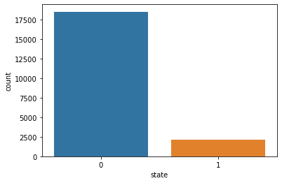
Only around 15% of Projects are granted.
In [8]:
np.log10(df1['goal_usd']).plot.hist(bins = 35)
plt.title('Logged Indiegogo Goals')
plt.xlabel('log10 Goal')
Out[8]:Text(0.5, 0, ‘log10 Goal’)
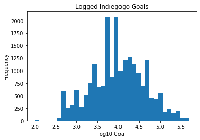
The goal dollar is in a normal distribution.
In [13]:
df1['log_goal'] = df1.loc[:, 'goal_usd'].apply(lambda l: np.log10(l+1))
plt.figure(figsize = (6,6))
sns.boxplot(x ='state', y = 'log_goal', data = df1)
plt.title('Successful Fundraiser have on average lower Goals')
df.groupby('state')['goal_usd'].median().T
Out[13]:state 0 10000.00000 1 12062.59975 Name: goal_usd, dtype: float64
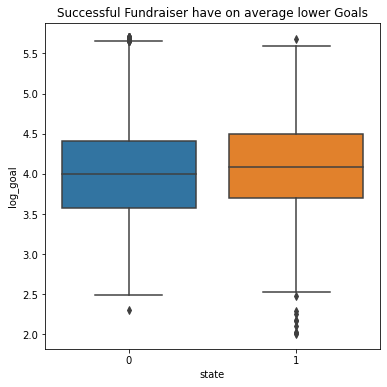
The median successful fundraiser had a goal of ‘10000USD’ while the median unsuccessful fundraiser had a goal of ‘12062USD’.
In [9]:
dfg = df1.groupby(['country', 'state']).size()
df1.groupby(['country', 'state']).size().unstack(fill_value=0).plot.bar()
plt.title("Number of fundraising in different country")
plt.xlabel('Country')
plt.ylabel('Number')
plt.legend(["Failure", "Success"])
plt.show()
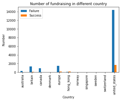
We can clearly see that most of the fundraising is from the united_states.
In [15]:
duration_values = df1.loc[:, 'fund_time'].unique()
per_duration_approved = {}
per_duration_count = {}
for dur in duration_values:
per_duration_approved[dur] = df1.loc[df1['fund_time'] == dur, 'state'].sum() / float((df1.loc[:, 'fund_time']==dur).sum())
per_duration_count[dur] = len(df1.loc[df1['fund_time'] == dur, 'state'])
plt.figure(figsize=(12, 5), dpi= 80)
ax = plt.subplot(1, 2, 2)
df1['log_goal'] = df1.loc[:, 'goal_usd'].apply(lambda l: np.log10(l+1))
df1.plot(kind='scatter', x='log_goal', y='fund_time', s = 2, alpha = 0.2, ax=ax, fontsize=10, colormap='Paired', c='state');
ax.set_xlabel('State (log $)', fontsize=12)
ax.set_ylabel('Duration (days)', fontsize=12)
plt.title('Goal is generally independent to duration')
plt.subplot(1, 2, 1)
plt.bar(list(per_duration_approved.keys()),list(per_duration_approved.values()), alpha = 0.5)
plt.xlabel('Duration (days)', fontsize=12)
plt.ylabel('% Funded', fontsize=12)
plt.title('Success rate as function of duration')
Out[15]:Text(0.5, 1.0, ‘Success rate as function of duration’)
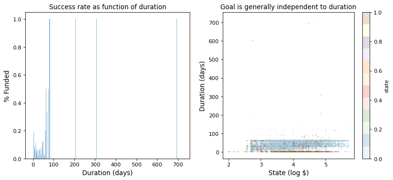
Little conclusion on the above two graph
- We can see that most of the fundraising event lasted for 0-100 days only.
- Goal USD (fundraising money) is generally independent to duration.
- As the sample data of those longer duration of the fundraising event are not enough, so we cannot really conclude that there is any relation between longer duration and higher success rate.
Module 3: Classification
In this step, I will evaluate different machine learning model performance in order to decide which one should be used in the next prediction module.
In [74]:
import sklearn
from sklearn import model_selection
from sklearn import preprocessing, svm
from sklearn.model_selection import train_test_split
from sklearn.linear_model import LinearRegression, LogisticRegression
from sklearn.naive_bayes import GaussianNB
from sklearn.tree import DecisionTreeClassifier
from sklearn.neighbors import KNeighborsClassifier
from sklearn.discriminant_analysis import LinearDiscriminantAnalysis
from sklearn.svm import SVC
from sklearn.ensemble import RandomForestClassifier
from sklearn.metrics import accuracy_score
from sklearn.datasets import make_regression
from sklearn.ensemble import RandomForestRegressor
In [20]:
final = df1[['country', 'category', 'state', 'goal_usd', 'fund_time']]
Out[20]:
| country | category | state | goal_usd | fund_time | |
|---|---|---|---|---|---|
| 0 | united_states | Transportation | 0 | 5000.0 | 21 |
| 1 | united_states | Human Rights | 0 | 1200.0 | 22 |
| 2 | united_states | Human Rights | 0 | 1200.0 | 22 |
| 3 | united_states | Photography | 0 | 2000.0 | 30 |
| 4 | united_states | Human Rights | 0 | 55000.0 | 120 |
First, I will have to change all the categorical data (string) into different value (integer) so that they can be processed.
In [34]:
def handle_non_numerical_data(df):
columns = final.columns.values
for column in columns:
text_digit_vals = {}
def convert_to_int(val):
return text_digit_vals[val]
if final[column].dtype != np.int64 and final[column].dtype != np.float64:
column_contents = final[column].values.tolist()
unique_elements = set(column_contents)
x = 0
for unique in unique_elements:
if unique not in text_digit_vals:
text_digit_vals[unique] = x
x+=1
final[column] = list(map(convert_to_int, final[column]))
return final
In [36]:
final = handle_non_numerical_data(final)
final.head()
Out[36]:
| country | category | state | goal_usd | fund_time | |
|---|---|---|---|---|---|
| 0 | 9 | 23 | 0 | 5000.0 | 21 |
| 1 | 9 | 21 | 0 | 1200.0 | 22 |
| 2 | 9 | 21 | 0 | 1200.0 | 22 |
| 3 | 9 | 0 | 0 | 2000.0 | 30 |
| 4 | 9 | 21 | 0 | 55000.0 | 120 |
So now, I will split the dataset into 70:30 ratio of training and testing tests. The former will be used for model training and the latter for evaluating the performance of the trained model.
In [52]:
X = np.array(final.drop(['state'],1))
y = np.array(final['state'])
print('Shape X: ', X.shape)
print('Shape y: ', y.shape)
X_train, X_test, y_train, y_test = train_test_split(X, y, test_size=0.3, random_state=666)
print('Train Shapes: ', X_train.shape, y_train.shape)
print('Test Shapes: ', X_test.shape, y_test.shape)
Shape X: (20631, 4) Shape y: (20631,) Train Shapes: (14441, 4) (14441,) Test Shapes: (6190, 4) (6190,)
Scale the data to fit the scaler
In [53]:
from sklearn.preprocessing import StandardScaler
scaler = StandardScaler()
X_train_scaled = scaler.fit_transform(X_train)
X_test_scaled = scaler.transform(X_test)
Apply Dimensional Reduction by using Principal Components Analysis (PCA)
I will use ‘n_componets=2’ as the original data has 4 columns (country, category, goal_usd, fund_time) and the code can project the original data into 2 dimensions only which can speed up the learning algorithm.
In [55]:
from sklearn.decomposition import PCA
pca = PCA(n_components=2)
X_train_dim_red = pca.fit_transform(X_train_scaled)
X_test_dim_red = pca.transform(X_test_scaled)
Model Evaluation
In [59]:
models = []
models.append(('CART', DecisionTreeClassifier()))
models.append(('NB', GaussianNB()))
models.append(('LDA', LinearDiscriminantAnalysis()))
models.append(('KNN', KNeighborsClassifier()))
models.append(('LR', LogisticRegression()))
models.append(('SVM', SVC(gamma='auto')))
models.append(('RFC', RandomForestClassifier()))
results = []
names = []
scoring = 'accuracy'
for name, model in models:
kfold = model_selection.KFold(n_splits = 10, shuffle = True, random_state = 666)
cv_results = model_selection.cross_val_score(model, X_train_dim_red, y_train, cv = kfold, scoring = scoring)
results.append(cv_results)
names.append(name)
result = "%s: %f (%f)" % (name, cv_results.mean(), cv_results.std())
print(result)
CART: 0.889343 (0.008686) NB: 0.897307 (0.006796) LDA: 0.897445 (0.007028) KNN: 0.912472 (0.005327) LR: 0.900907 (0.007321) SVM: 0.913787 (0.007752) RFC: 0.912540 (0.006731)
Although Support Vector Classification got the highest accuracy from fitting our data, the speed of it is way too slow. So I will use RandomForestClassifier instead.
Module 4: Prediction
In this part, I am going to use RandomForestCleassifier model to predict the outcome of whether Indiegogo fundraise was success or not.
In [66]:
clf = RandomForestClassifier()
clf = clf.fit(X_train_dim_red, y_train)
Y_pred = clf.predict(DecisionTreeClassifier())
In [67]:
prediction = clf.predict(X_test_dim_red)
print('prediction: ', prediction)
type(prediction)
prediction: [0 0 0 … 0 0 0]
Out[67]:numpy.ndarray
In [71]:
model = RandomForestClassifier()
model.fit(X_train_dim_red, y_train)
predictions = model.predict(X_test_dim_red)
print(f'Model Accuracy: {accuracy_score(y_test, predictions):.2f}')
Model Accuracy: 0.91
Random Forest Classifier Feature Importance
Because of the feature is being reduced into 2 when using Principal Components Analysis so I have to use the original non-scaled data to process the model again in order to get the feature importance rank of all 4 features.
In [94]:
# define the new model
new_model = RandomForestClassifier()
# fit the model
new_model.fit(X_train, y_train)
# get importance
importance = new_model.feature_importances_
# summarize feature importance
for i,v in enumerate(importance):
    print('Feature: %0d, Score: %.5f' % (i,v))
Feature: 0, Score: 0.05462 Feature: 1, Score: 0.11225 Feature: 2, Score: 0.41621 Feature: 3, Score: 0.41691
In [95]:
feats = {} # a dict to hold feature_name: feature_importance
final_df = final.drop(['state'],1)
for feature, importance in zip(final_df.columns,
new_model.feature_importances_):
feats[feature] = importance #add the name/value pair
importances = pd.DataFrame.from_dict(feats, orient="index").rename(columns={0: 'Gini-importance'})
importances.sort_values(by='Gini-importance').plot(kind='barh',figsize=(10,8))
Out[95]:<AxesSubplot:>
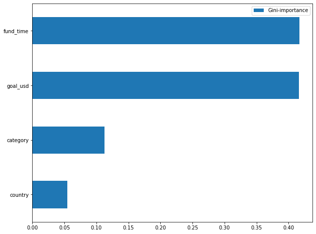
For more convient to see which feature best affecting the result in the model, I have made a new graph that use the feature names directly.
Module 5: Summary
I am going to summarize my findings and draw conclusions by using Q and A format. So that this chance of experience can be better recorded.
Q: What have you done and what have you learned?
A: So basically to conclude what I have done, I have to understand the property of the given data first so that I can start building up the plan to analyze it which is all the stuff you can see in module 1. Then, I will go deeper into the data like visualizing different variables with the target value by plotting graph. It gives me some insight like whether the dataset is linearly separable so that the result will be much easier to predict in the later module. In the process of doing all of this, you can see that I keep adjusting the dataset so that it fits my requirement to finish certain tasks. For example, without scaling the data to fit the scaler, the model may not be that easy to learn and understand the problem as the values of the features are not that close to each other, the algorithm may become slower. Therefore, before the process of the dimension reduction and classification, I have applied some of the skills I learnt from the tutorials like I have to encode all the categorical items first so that the model can process it easily. Apart from that, I use quite a lot of time on reading docs of some function and the library. Except from the offical docs, I found stackoverflow and geeksforgeeks provided me many useful resources as well. This experience can certainly conslidate my coding skills and logic flow.
Q: What is the biggest difficuly in this project and how did you solve it?
A: Undoubtedly, everytime when I have to answer this question, I would say module 2 is the most challenging parts for me. As this module requires me to interpret it step by step, you cannot always plot the exact graph that give you insight on what is the next step, so it takes a lot of time to discover and explore it yourself. The dataset itself doesn’t give me any hints of finding the relation between feautres(variables) and objects(class). So I have to base on my little experience to plot graph myself to find something useful as there isn’t any fixed standard working flow on it. I stucked in this part for quite long after plotting many different graphs, but I turned out understand that not always there will be lots of big discoveries when you are trying to explore a new dataset. You have to understand that sometimes finding something simple doesn’t mean you have not done anything, it is also a part of exploration and analyzing result. There is not always a fixed solution for a problem, data only gives you insight on how you can use it to prove your view.
Q: What do you think of annotation, how does it helps?
A: I have annotate each part steps by steps in order to let the readers understand what is that part doing. It helps me to debug as I can find the problem of code quickly with those annotation. And when I try to present it to any other, I can share it with more clearer steps as everything was done in order.
Q: How you finish solving this project?
A: My basic flow of solving quesion and doing analysis is writing all steps onto a paper first. During the progress, I have to further brainstorm the possibility of doing wrong or missing important factors, so I will always think of what I am going to do in this coming module and strictly follow the procedures so that I won’t digress from the progress and don’t know what I am doing and what I have to do.
Q: What are the main results?
A: As I stated above, Support Vector Machines is currently the best performing model among the models I have tested, and the probability of Random Forest classifying positive samples on the test set is pretty high too which is over 91%.
Q: From the result, what have you discovered?
A: In my opinion, it seems that the overall funding time and the money to raise affecting the success rate of a fundraising event the most as it also proved our assumption that it is totally possible to predict the state of a campaign by only using the duration and the goal of the event.
