This is an individual project of SDSC2001 – Python for Data Science. I did the project in my year 2 2021/22 Semester A.
Course Instructor: Professor LI Xinyue
Context
Credit card companies aim to recognize fraudulent credit card transactions so that customers are not charged for items that they did not purchase.
Content
The dataset contains transactions made by credit cards in September 2013 by european cardholders. Transactions occurred in two days, where we have 492 frauds out of 284,807 transactions. The dataset is highly unbalanced, as the positive class (frauds) account for 0.172% of all transactions.
It contains numerical input variables V1-V28 which are the result of a Principal Component Analysis (PCA) transformation, as original features are not provided due to confidentiality issues. Features that have not been transformed with PCA are ‘Time’ and ‘Amount’. ‘Time’ contains the seconds elapsed between each transaction and the first transaction in the dataset. ‘Amount’ denotes the transaction Amount. ‘Class’ is the response variable (labelled outcome) and it takes value 1 in case of fraud and 0 otherwise.
Module 1: Data Exploration
In [1]:
# define all library that I may need to use
import matplotlib.pyplot as plt
import numpy as np
import pandas as pd
import seaborn as sns
import warnings
warnings.simplefilter(action='ignore', category=FutureWarning)
pd.options.mode.chained_assignment = None  # remove warning
from collections import Counter
In [2]:
# load the csv file into a data frame and show the first 5 rows in order to have a quick look on the data
df = pd.read_csv ('creditcard_train.csv')
df.head()
Out[2]:
| Time | V1 | V2 | V3 | V4 | V5 | V6 | V7 | V8 | V9 | … | V21 | V22 | V23 | V24 | V25 | V26 | V27 | V28 | Amount | Class | |
|---|---|---|---|---|---|---|---|---|---|---|---|---|---|---|---|---|---|---|---|---|---|
| 0 | 0.0 | -1.359807 | -0.072781 | 2.536347 | 1.378155 | -0.338321 | 0.462388 | 0.239599 | 0.098698 | 0.363787 | … | -0.018307 | 0.277838 | -0.110474 | 0.066928 | 0.128539 | -0.189115 | 0.133558 | -0.021053 | 149.62 | 0 |
| 1 | 0.0 | 1.191857 | 0.266151 | 0.166480 | 0.448154 | 0.060018 | -0.082361 | -0.078803 | 0.085102 | -0.255425 | … | -0.225775 | -0.638672 | 0.101288 | -0.339846 | 0.167170 | 0.125895 | -0.008983 | 0.014724 | 2.69 | 0 |
| 2 | 1.0 | -1.358354 | -1.340163 | 1.773209 | 0.379780 | -0.503198 | 1.800499 | 0.791461 | 0.247676 | -1.514654 | … | 0.247998 | 0.771679 | 0.909412 | -0.689281 | -0.327642 | -0.139097 | -0.055353 | -0.059752 | 378.66 | 0 |
| 3 | 1.0 | -0.966272 | -0.185226 | 1.792993 | -0.863291 | -0.010309 | 1.247203 | 0.237609 | 0.377436 | -1.387024 | … | -0.108300 | 0.005274 | -0.190321 | -1.175575 | 0.647376 | -0.221929 | 0.062723 | 0.061458 | 123.50 | 0 |
| 4 | 2.0 | -1.158233 | 0.877737 | 1.548718 | 0.403034 | -0.407193 | 0.095921 | 0.592941 | -0.270533 | 0.817739 | … | -0.009431 | 0.798278 | -0.137458 | 0.141267 | -0.206010 | 0.502292 | 0.219422 | 0.215153 | 69.99 | 0 |
In [3]:
# find out the total number of rows and columns in the file
print(df.shape)
# it seems there are some data missing, lets try to solve it!
Out[3]: (284657, 31)
In [4]:
# So first, we have to find out where and how many are the missing data
df.isnull().sum()
Out[4]:Time 0 V1 0 V2 0 V3 0 V4 0 V5 0 V6 0 V7 0 V8 0 V9 0 V10 0 V11 0 V12 0 V13 0 V14 0 V15 0 V16 0 V17 0 V18 0 V19 0 V20 0 V21 0 V22 278 V23 520 V24 0 V25 0 V26 0 V27 0 V28 0 Amount 0 Class 0 dtype: int64
In [5]:
missing_col = ['V22','V23']
#Using mean and looping to impute the missing values
for i in missing_col:
    df.loc[df.loc[:,i].isnull(),i] = df.loc[:,i].mean()
In [6]:
#After filling missing data, we have to detect the outliers and remove them, except the result
Q1 = df.iloc[:,:-1].quantile(0.25)
Q3 = df.iloc[:,:-1].quantile(0.75)
IQR = Q3 - Q1
data = df[~((df < (Q1 - 2.5 * IQR)) | (df > (Q3 + 2.5 * IQR))).any(axis=1)]
print(data.shape)
(213174, 31)
In [7]:
#I want to see some basic info of the data for later data visualization
#like mean of time..., in order to see is there any insight
data.describe().T
Out[7]:
| count | mean | std | min | 25% | 50% | 75% | max | |
|---|---|---|---|---|---|---|---|---|
| Time | 213174.0 | 95141.575281 | 47383.880288 | 0.000000 | 54623.500000 | 84469.000000 | 139655.000000 | 172792.000000 |
| V1 | 213174.0 | 0.496082 | 1.276026 | -5.536010 | -0.618926 | 0.999862 | 1.718921 | 2.454930 |
| V2 | 213174.0 | 0.079463 | 0.827586 | -4.098951 | -0.463757 | 0.068991 | 0.703425 | 3.808020 |
| V3 | 213174.0 | 0.164240 | 1.260900 | -4.846779 | -0.679702 | 0.286612 | 1.088969 | 4.079168 |
| V4 | 213174.0 | 0.001365 | 1.283098 | -4.826127 | -0.784687 | 0.031907 | 0.703920 | 4.720074 |
| V5 | 213174.0 | -0.024155 | 0.910768 | -3.252559 | -0.621899 | -0.070961 | 0.492316 | 3.870056 |
| V6 | 213174.0 | -0.205544 | 0.897459 | -3.666150 | -0.786134 | -0.351098 | 0.189226 | 3.315460 |
| V7 | 213174.0 | 0.011357 | 0.712423 | -3.180199 | -0.494948 | 0.044931 | 0.513259 | 3.008217 |
| V8 | 213174.0 | 0.076681 | 0.381320 | -1.548042 | -0.170941 | 0.022833 | 0.266917 | 1.666501 |
| V9 | 213174.0 | -0.041198 | 0.975211 | -3.672923 | -0.621874 | -0.062938 | 0.535013 | 3.695086 |
| V10 | 213174.0 | -0.047962 | 0.738765 | -2.999375 | -0.502612 | -0.104048 | 0.342025 | 2.926167 |
| V11 | 213174.0 | 0.002681 | 0.991865 | -3.241392 | -0.772031 | -0.006187 | 0.757923 | 3.531399 |
| V12 | 213174.0 | 0.044023 | 0.856469 | -2.964042 | -0.369406 | 0.161963 | 0.625702 | 2.601809 |
| V13 | 213174.0 | -0.008020 | 1.012035 | -3.888606 | -0.686500 | -0.010238 | 0.683467 | 3.904562 |
| V14 | 213174.0 | 0.018659 | 0.743759 | -2.720881 | -0.397002 | 0.048117 | 0.453591 | 2.788031 |
| V15 | 213174.0 | -0.012136 | 0.889419 | -3.657525 | -0.576125 | 0.036738 | 0.622986 | 3.601890 |
| V16 | 213174.0 | 0.017735 | 0.779686 | -2.944460 | -0.430518 | 0.076966 | 0.500815 | 2.686354 |
| V17 | 213174.0 | -0.037677 | 0.629111 | -2.311921 | -0.487001 | -0.093053 | 0.345882 | 2.606673 |
| V18 | 213174.0 | -0.021883 | 0.791908 | -2.997391 | -0.505811 | -0.029341 | 0.460010 | 2.997719 |
| V19 | 213174.0 | 0.002176 | 0.733705 | -2.743833 | -0.409821 | 0.016457 | 0.437332 | 2.744196 |
| V20 | 213174.0 | -0.068025 | 0.229977 | -1.073139 | -0.206210 | -0.084503 | 0.064950 | 0.993129 |
| V21 | 213174.0 | -0.025548 | 0.259462 | -1.251701 | -0.221372 | -0.038575 | 0.155363 | 1.222562 |
| V22 | 213174.0 | 0.003638 | 0.674379 | -2.659080 | -0.542021 | 0.009103 | 0.513472 | 2.471164 |
| V23 | 213174.0 | -0.000756 | 0.215954 | -0.933712 | -0.133954 | -0.006191 | 0.129913 | 0.921028 |
| V24 | 213174.0 | -0.026047 | 0.575898 | -2.337548 | -0.364409 | 0.028063 | 0.401640 | 1.307137 |
| V25 | 213174.0 | 0.003608 | 0.462133 | -1.986743 | -0.305288 | 0.019155 | 0.341251 | 1.966419 |
| V26 | 213174.0 | -0.001525 | 0.461604 | -1.641329 | -0.316247 | -0.038658 | 0.222019 | 1.660394 |
| V27 | 213174.0 | 0.021914 | 0.145059 | -0.475451 | -0.055080 | 0.004869 | 0.078575 | 0.495576 |
| V28 | 213174.0 | 0.012159 | 0.102029 | -0.380841 | -0.045706 | 0.009546 | 0.056236 | 0.405955 |
| Amount | 213174.0 | 41.932054 | 53.786545 | 0.000000 | 4.990000 | 18.910000 | 57.200000 | 256.000000 |
| Class | 213174.0 | 0.000145 | 0.012058 | 0.000000 | 0.000000 | 0.000000 | 0.000000 | 1.000000 |
Module 2: Data Visualization
In [8]:
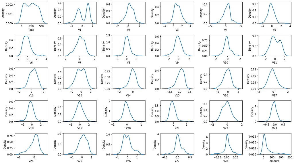
#First graph, I have to see hows the distributions of all variable
fig,ax=plt.subplots(5,6,figsize=[16,9])
columns=data.columns
for idx,ax in enumerate(ax.flat):
    sns.kdeplot(data.loc[:,columns[idx]][:500],ax=ax)
plt.tight_layout()
#As the data has removed the outliers, but after plotting all the graph,
#we can see that it is not Normalized and Standardized
#so we may consider to apply normalization into the data
In [9]:
#applying Normalization from sklearn library by using minmaxscaler
from sklearn.preprocessing import MinMaxScaler
scaler = MinMaxScaler()
scaler.fit(data.iloc[:,:-1])
data.iloc[:,:-1]=scaler.transform(data.iloc[:,:-1])
In [10]:
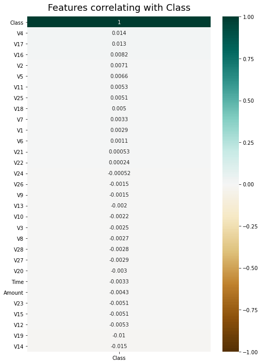
#Second graph, we have to see are there any features ('Variables') have correlation with our object ('Class')
plt.figure(figsize=(8, 12))
heatmap = sns.heatmap(data.corr()[['Class']].sort_values(by='Class', ascending=False), vmin=-1, vmax=1, annot=True, cmap='BrBG')
heatmap.set_title('Features correlating with Class', fontdict={'fontsize':18}, pad=12)
plt.show()
#After plotting the heatmap, we can concluded all the corrleation are very low.
In [11]:
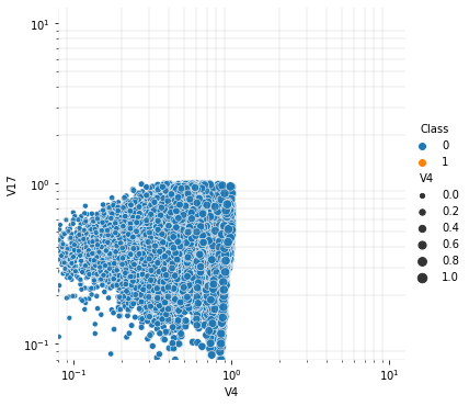
#As the info we got right now aren't very useful, we still can't make any assumption
#then we can only try to visualize the highest correlation between the two variables and class to see is there any useful info
cmap = sns.cubehelix_palette(rot=-.2, as_cmap=True)
g=sns.relplot(
    data=data,
    x="V4", y="V17",
    hue="Class", size="V4",
)
g.set(xscale="log", yscale="log")
g.ax.xaxis.grid(True, "minor", linewidth=.25)
g.ax.yaxis.grid(True, "minor", linewidth=.25)
g.despine(left=True, bottom=True)
plt.show()
#After ploting the scatterplot,
#it seems that there is a serious problem of unbalanced sample size which greatly affect my assumption
#also we can conclude that it cannot be divided by the variables(V4 V17) alone class(0 1) category
In [12]:
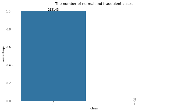
#Further investigating of the problem of unbalanced sample size by plotting the number of normal and fraudulent cases out
fig,ax=plt.subplots(figsize=[10,6])
bar=data.Class.value_counts()
sns.barplot(x=bar.index,y=bar.values/len(data),ax=ax)
plt.title('The number of normal and fraudulent cases')
plt.xlabel('Class')
plt.ylabel('Percentage')
for y,x  in enumerate(bar.values/len(data)):
    plt.text(y,x,s=bar[y],va='bottom',ha='center')
plt.show()
#As now, we can conclude the sample size are highly unbalanced,
#I have done a similar analysis on p2p debit and credit risk, the ratio is 1:49
#But this dataset, only have 0.014% positive sample size (fraudulent)
#it is way more less than the given percentage 0.172%
#maybe it is my problem that some important data are being removed during the process of data cleaning
#Currently, I am pessimistic about this model
Module 3: Dimension Reduction
In [13]:
#We will use principal component analysis from sklearn library to achieve dimension reduction
from sklearn.decomposition import PCA
pca=PCA(n_components=2).fit(data.iloc[:,:-1]) #remove 'Class' column and compress the data into 2d
features_pca=pca.transform(data.iloc[:,:-1])
In [14]:
#have some basic view with the principal component
features_pca
Out[14]:array([[ 6.65811147e-01, 1.89550269e-01], [ 4.93164830e-01, -3.89688202e-04], [ 5.96507876e-01, 1.64345532e-01], …, [-3.12209498e-01, -2.19958181e-01], [-5.22941908e-01, 6.27902788e-02], [-4.04661011e-01, 2.29348807e-01]])
In [15]:
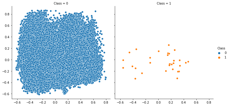
sns.relplot(x=features_pca[:,0],y=features_pca[:,1],hue=data.Class,col=data.Class)
plt.show()
#As the positive and negative sample size are unbalanced, it is difficult to show them on single graph
#so we have to divide them into two
#Now, we can conclude that this is a linearly inseparable problem.
#It is very difficult for us to find a decision boundary to separate the categories of 0 and 1.
Module 4: Classification
In [16]:
###pick 3 classification methods, and methods not in the below list can also be used
from sklearn.linear_model import LogisticRegression
from sklearn.discriminant_analysis import LinearDiscriminantAnalysis
from sklearn.discriminant_analysis import QuadraticDiscriminantAnalysis
from sklearn.neighbors import KNeighborsClassifier
from sklearn.tree import DecisionTreeClassifier
from sklearn.svm import SVC
from sklearn.ensemble import RandomForestClassifier, AdaBoostClassifier
from sklearn.naive_bayes import GaussianNB
from sklearn.gaussian_process import GaussianProcessClassifier
from sklearn.gaussian_process.kernels import RBF
In [17]:
#Before doing classification and modelling,
#we have to do some preparation on our data first in order to solve the undersampling problem.
#First, we filter out all the positive sample.
pos=data.loc[data.Class==1]
pos.head()
Out[17]:
| Time | V1 | V2 | V3 | V4 | V5 | V6 | V7 | V8 | V9 | … | V21 | V22 | V23 | V24 | V25 | V26 | V27 | V28 | Amount | Class | |
|---|---|---|---|---|---|---|---|---|---|---|---|---|---|---|---|---|---|---|---|---|---|
| 10471 | 0.099466 | 0.828987 | 0.632028 | 0.587217 | 0.837651 | 0.481326 | 0.493320 | 0.510181 | 0.478192 | 0.615223 | … | 0.334705 | 0.362210 | 0.545266 | 0.687345 | 0.591153 | 0.461089 | 0.502971 | 0.552996 | 0.014805 | 1 |
| 10484 | 0.099657 | 0.841677 | 0.637569 | 0.552223 | 0.822335 | 0.514553 | 0.494404 | 0.522550 | 0.447245 | 0.618447 | … | 0.302743 | 0.314153 | 0.472821 | 0.547883 | 0.639483 | 0.467340 | 0.486505 | 0.547359 | 0.014805 | 1 |
| 14319 | 0.147148 | 0.833612 | 0.661327 | 0.435114 | 0.785843 | 0.595657 | 0.490264 | 0.564990 | 0.519826 | 0.343319 | … | 0.438500 | 0.416578 | 0.442831 | 0.478909 | 0.634311 | 0.510243 | 0.505249 | 0.564889 | 0.014687 | 1 |
| 27339 | 0.199784 | 0.828093 | 0.571061 | 0.639674 | 0.769624 | 0.455947 | 0.605805 | 0.493959 | 0.550985 | 0.407074 | … | 0.441471 | 0.458833 | 0.532329 | 0.644585 | 0.597468 | 0.464918 | 0.511272 | 0.497461 | 0.005938 | 1 |
| 50497 | 0.257720 | 0.663387 | 0.563346 | 0.763948 | 0.374027 | 0.360987 | 0.429760 | 0.523447 | 0.480594 | 0.650837 | … | 0.595075 | 0.696105 | 0.349038 | 0.765157 | 0.550207 | 0.336032 | 0.616497 | 0.534346 | 0.003906 | 1 |
In [18]:
#We have to generate some random sample for later classification use
np.random.seed(1234)
data=data.sample(frac=1) #Return a random sample of data.
neg=data.loc[data.Class==0][:len(pos)] #Select negative samples with the same number of positive samples
neg.head()
Out[18]:
| Time | V1 | V2 | V3 | V4 | V5 | V6 | V7 | V8 | V9 | … | V21 | V22 | V23 | V24 | V25 | V26 | V27 | V28 | Amount | Class | |
|---|---|---|---|---|---|---|---|---|---|---|---|---|---|---|---|---|---|---|---|---|---|
| 126992 | 0.452561 | 0.862580 | 0.427405 | 0.549750 | 0.420335 | 0.417202 | 0.659959 | 0.391111 | 0.538233 | 0.410159 | … | 0.308037 | 0.388702 | 0.434289 | 0.294569 | 0.606618 | 0.844428 | 0.468568 | 0.462663 | 0.058594 | 0 |
| 183343 | 0.728060 | 0.903462 | 0.402517 | 0.606008 | 0.665632 | 0.291794 | 0.659313 | 0.302441 | 0.626403 | 0.740388 | … | 0.609877 | 0.702927 | 0.524760 | 0.534089 | 0.440702 | 0.338447 | 0.593475 | 0.461779 | 0.343711 | 0 |
| 64620 | 0.296617 | 0.844377 | 0.522574 | 0.650733 | 0.624634 | 0.390661 | 0.568212 | 0.434091 | 0.504582 | 0.602396 | … | 0.464229 | 0.512938 | 0.436808 | 0.525002 | 0.646065 | 0.387843 | 0.571280 | 0.525252 | 0.039023 | 0 |
| 38807 | 0.229021 | 0.819414 | 0.525336 | 0.581708 | 0.656817 | 0.442502 | 0.508198 | 0.557331 | 0.445715 | 0.507953 | … | 0.490752 | 0.521458 | 0.423099 | 0.679017 | 0.674914 | 0.398378 | 0.524619 | 0.525879 | 0.344023 | 0 |
| 112818 | 0.421570 | 0.618444 | 0.673766 | 0.644609 | 0.540979 | 0.414852 | 0.398353 | 0.639453 | 0.526851 | 0.347534 | … | 0.390898 | 0.315202 | 0.699672 | 0.748187 | 0.304074 | 0.486842 | 0.461561 | 0.617672 | 0.241602 | 0 |
In [19]:
#Concatenate the positive and negative data and read the test set
train=pd.concat([pos,neg])
test=pd.read_csv ('creditcard_test.csv')
test.head()
Out[19]:
| Time | V1 | V2 | V3 | V4 | V5 | V6 | V7 | V8 | V9 | … | V21 | V22 | V23 | V24 | V25 | V26 | V27 | V28 | Amount | Class | |
|---|---|---|---|---|---|---|---|---|---|---|---|---|---|---|---|---|---|---|---|---|---|
| 0 | 40086 | 1.083693 | 1.179501 | -1.346150 | 1.998824 | 0.818034 | -0.771419 | 0.230307 | 0.093683 | -0.167594 | … | -0.312000 | -0.639700 | -0.120249 | -0.180218 | 0.609283 | -0.339524 | 0.096701 | 0.114972 | 1.00 | 1 |
| 1 | 93860 | -10.850282 | 6.727466 | -16.760583 | 8.425832 | -10.252697 | -4.192171 | -14.077086 | 7.168288 | -3.683242 | … | 2.541637 | 0.135535 | -1.023967 | 0.406265 | 0.106593 | -0.026232 | -1.464630 | -0.411682 | 78.00 | 1 |
| 2 | 14152 | -4.710529 | 8.636214 | -15.496222 | 10.313349 | -4.351341 | -3.322689 | -10.788373 | 5.060381 | -5.689311 | … | 1.990545 | 0.223785 | 0.554408 | -1.204042 | -0.450685 | 0.641836 | 1.605958 | 0.721644 | 1.00 | 1 |
| 3 | 27219 | -25.266355 | 14.323254 | -26.823673 | 6.349248 | -18.664251 | -4.647403 | -17.971212 | 16.633103 | -3.768351 | … | 1.780701 | -1.861318 | -1.188167 | 0.156667 | 1.768192 | -0.219916 | 1.411855 | 0.414656 | 99.99 | 1 |
| 4 | 84204 | -1.927453 | 1.827621 | -7.019495 | 5.348303 | -2.739188 | -2.107219 | -5.015848 | 1.205868 | -4.382713 | … | 1.376938 | -0.792017 | -0.771414 | -0.379574 | 0.718717 | 1.111151 | 1.277707 | 0.819081 | 512.25 | 1 |
In [20]:
#Perform the same data transformation on the test set
test.iloc[:,:-1]=scaler.transform(test.iloc[:,:-1])
test.head()
Out[20]:
| Time | V1 | V2 | V3 | V4 | V5 | V6 | V7 | V8 | V9 | … | V21 | V22 | V23 | V24 | V25 | V26 | V27 | V28 | Amount | Class | |
|---|---|---|---|---|---|---|---|---|---|---|---|---|---|---|---|---|---|---|---|---|---|
| 0 | 0.231990 | 0.828401 | 0.667569 | 0.392186 | 0.714939 | 0.571503 | 0.414622 | 0.551111 | 0.510718 | 0.475750 | … | 0.379791 | 0.393623 | 0.438586 | 0.591911 | 0.656696 | 0.394280 | 0.589224 | 0.630167 | 0.003906 | 1 |
| 1 | 0.543196 | -0.665037 | 1.369224 | -1.334738 | 1.388192 | -0.982804 | -0.075344 | -1.760852 | 2.711530 | -0.001401 | … | 1.533118 | 0.544733 | -0.048662 | 0.752826 | 0.529535 | 0.489168 | -1.018694 | -0.039198 | 0.304688 | 1 |
| 2 | 0.081902 | 0.103302 | 1.610625 | -1.193088 | 1.585916 | -0.154267 | 0.049195 | -1.229422 | 2.055789 | -0.273668 | … | 1.310389 | 0.561935 | 0.802334 | 0.311003 | 0.388564 | 0.691507 | 2.143513 | 1.401232 | 0.003906 | 1 |
| 3 | 0.157525 | -2.469089 | 2.329869 | -2.462136 | 1.170662 | -2.163769 | -0.140548 | -2.390113 | 5.655904 | -0.012952 | … | 1.225578 | 0.155502 | -0.137192 | 0.684343 | 0.949856 | 0.430506 | 1.943618 | 1.011059 | 0.390586 | 1 |
| 4 | 0.487314 | 0.451581 | 0.749538 | -0.243416 | 1.065809 | 0.072076 | 0.223291 | -0.296627 | 0.856703 | -0.096334 | … | 1.062393 | 0.363933 | 0.087504 | 0.537213 | 0.684379 | 0.833650 | 1.805468 | 1.525073 | 2.000977 | 1 |
In [21]:
#import cross-validation from sklearn library
from sklearn.model_selection import GridSearchCV
from sklearn.metrics import plot_confusion_matrix,classification_report
In [22]:
#train our data
train_y=train.pop('Class')
train_x=train
test_y=test.pop('Class')
test_x=test
In [23]:
#build a function that uses for training and evaluating different models, using 5-fold cross-validation
def train_and_evaluate(model,params):
    gs=GridSearchCV(model(random_state=1234),
                 param_grid=params, cv=5).fit(train_x,train_y)
    print('Train score :',gs.best_score_)
    print('Test score :',gs.score(test_x,test_y))
    plot_confusion_matrix(gs, test_x, test_y)
    plt.show()
    print(classification_report(test_y,gs.predict(test_x)))
    return gs
4.1 Training with RandomForestClassifier
In [24]:
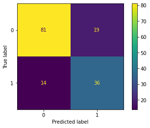
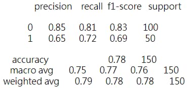
m1=train_and_evaluate(RandomForestClassifier,
                   params={'n_estimators':np.arange(10,40,5),
                          'max_features':np.arange(10,20,1)})
Train score : 0.8397435897435898 Test score : 0.78
4.2 Training with LogisticRegression
In [25]:
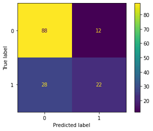
m2=train_and_evaluate(LogisticRegression,
                   params={
                          'C':np.linspace(0.1,1,10)}
                           )
Train score : 0.7371794871794872 Test score : 0.7333333333333333
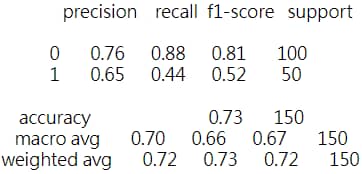
4.3 Training with Support Vector Machine
In [26]:
m3=train_and_evaluate(SVC,
                   params={
                          'C':np.arange(1,10,1),
                          'gamma':np.linspace(0.01,0.1,10)
                   }
                           )
Train score : 0.7717948717948718 Test score : 0.66
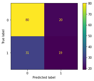
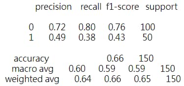
In [27]:
#After we have realised that the best model among these three should be random forest,
#we sort out most relevant features ranking
pd.DataFrame({'Feature':train_x.columns,
             'Value':m1.best_estimator_.feature_importances_}).sort_values(by='Value',ascending=False)
Out[27]:
| Feature | Value | |
|---|---|---|
| 14 | V14 | 0.218701 |
| 17 | V17 | 0.125888 |
| 4 | V4 | 0.111668 |
| 19 | V19 | 0.084166 |
| 16 | V16 | 0.065130 |
| 29 | Amount | 0.052899 |
| 15 | V15 | 0.038870 |
| 13 | V13 | 0.038309 |
| 27 | V27 | 0.034972 |
| 2 | V2 | 0.027462 |
| 28 | V28 | 0.022460 |
| 8 | V8 | 0.022411 |
| 23 | V23 | 0.018893 |
| 20 | V20 | 0.018022 |
| 6 | V6 | 0.016508 |
| 5 | V5 | 0.012932 |
| 0 | Time | 0.012430 |
| 18 | V18 | 0.011545 |
| 26 | V26 | 0.009688 |
| 9 | V9 | 0.009620 |
| 10 | V10 | 0.009097 |
| 22 | V22 | 0.007824 |
| 11 | V11 | 0.007375 |
| 12 | V12 | 0.006643 |
| 7 | V7 | 0.004063 |
| 1 | V1 | 0.003455 |
| 25 | V25 | 0.003063 |
| 21 | V21 | 0.002532 |
| 24 | V24 | 0.001935 |
| 3 | V3 | 0.001440 |
Module 5: Summary
I am going to summarize my findings and draw conclusions by using Q and A format. So that this chance of experience can be better recorded.
Q: What have you done and what have you learned?
A: So basically to conclude what I have done, I have to understand the property of the given data first so that I can start building up the plan to analyze it which is all the stuff you can see in module 1. Then, I will go deeper into the data like visualizing different variables with the target value by plotting graph. Although it may not really work just like this time, at least it still gives me some insight like the problem is linearly inseparable so that I can solve it with different method. In the process of doing all of this, you can see that I keep adjusting the dataset so that it fits my requirement to finish certain tasks. For example, without removing outliers, the accuracy of the model must be affected so all the steps I have done are effective and useful for the entire project. In the dimension reduction and classification, I have applied the skills I learnt from letures and tutorials. Apart from that, I use quite a lot of time on reading docs of some function and the library. Except from the offical docs, I found stackerflow and geeksforgeeks provided me many useful resources as well. This experience can certainly conslidate my coding skills and logic flow.
Q: What is the biggest difficuly in this project and how did you solve it?
A: Undoubtedly, I would say module 2 is the most challenging parts for me. As there isn’t many instructions on this module which gives me more freedom to interpret it, the dataset itself doesn’t give me any hints of finding the relation between feautres(variables) and objects(class). So I stucked in this part for quite long after plotting many different graphs, but I turned out understand that not always there is a big relationship between a single variable and a target. You have to know that sometimes finding them doesn’t have great relation is also a part of exploration and analyzing result. There is no fixed solution for a problem, data only gives you insight on how you can use it to prove your view.
Q: What do you think of annotation, how does it helps?
A: I have annotate each part steps by steps in order to let the readers understand what is that part doing. It helps me to debug as I can find the problem of code quickly with those annotation.
Q: How you finish solving this project?
A: My basic flow of solving quesion and doing analysis is writing all steps onto a paper first. During the progress, I have to further brainstorm the possibility of doing wrong or missing important factors, so if there are any hints that can be followed, then I will strictly follow the given procedures so that I won’t digress from the topic and don’t know what I am doing.
Q: What are the main results?
A: As I stated above, Random forest is currently the best performing model among the models I have tested, but the probability of classifying positive samples on the test set is the same as logistic regression, which is only 65%.
Q: From the result, what have you discovered?
A: In my opinion, this kind of fraud detection is obviously more important to correctly classify a positive sample than to classify a negative sample. It is because if you judge a negative sample as a positive sample, it may cause economic losses for the client and the company.
Q: What advice you can give to the credit card company?
A: If you want to avoid this situation, you need to increase the weight of the positive samples, but after doing so, more negative samples will be classified into positive samples, thus rejecting more customers to apply for credit cards. And there will also be a lose of profit. As a result, in order to find a balance, it really depends on how your company choose between risks and profits.
